Optimize Slow Data Queries With Doris JOIN Strategies

In the world of data analysis, "slow queries" are like workplace headaches that just won't go away.
Recently, I've met quite a few data analysts who complain about queries running for hours without results, leaving them staring helplessly at the spinning progress bar. Last week, I ran into an old friend who was struggling with the performance of a large table JOIN.

"The query speed is slower than a snail, and my boss is driving me crazy..." he said with a frustrated look.
As a seasoned database optimization expert with years of experience on the front lines, I couldn't help but smile: "JOIN performance is slow because you don't understand its nature. Just like in martial arts, understanding how to use force effectively can make all the difference."

Today, let's dive into the world of JOIN operations in Doris and see how you can transform your queries into "lightning-fast" operations that will impress your boss!

Doris JOIN Secret: Performance Optimization Starts With Choosing the Right JOIN Strategy

Data Analyst Xiao Zhang recently encountered a tricky problem. He was working on a large-scale data analysis task that required joining several massive tables. Initially, he used the most conventional JOIN method, but the query speed was painfully slow, taking hours to complete. This left him in a tough spot — his boss needed the report urgently, and the pressure was mounting.

Xiao Zhang turned to his old friend and Doris expert, Old Li, for help. Old Li smiled and said, "The key to JOIN performance is choosing the right JOIN strategy. Doris supports multiple JOIN implementations, and I'll share some secrets with you."

The Essence of JOIN

In distributed databases, JOIN operations may seem simple, but they actually involve hidden complexities. They not only need to join tables but also coordinate data flow and computation in a distributed environment.

For example, you have two large tables distributed across different nodes, and to perform a JOIN, you need to solve a core problem — how to bring the data to be joined together. This involves data redistribution strategies.

Doris' JOIN Arsenal

Doris employs two main physical implementations for JOIN operations — Hash Join and Nest Loop Join. Hash Join is like a martial artist's swift sword, completing joins with lightning speed; Nest Loop Join is like a basic skill for a swordsman, simple but widely applicable.

Hash Join builds a hash table in memory and can quickly complete equi-JOIN operations. It's like finding teammates in a game of League of Legends — each player is assigned a unique ID, and when needed, the system locates them directly, naturally achieving high efficiency.

Nest Loop Join, on the other hand, uses the most straightforward method — iteration. It's like visiting relatives during the Spring Festival, going door-to-door, which is slower but ensures that no one is missed. This method is applicable to all JOIN scenarios, including non-equi-JOINs.

The Four Data Distribution Strategies in the JOIN World

As a distributed MPP database, Apache Doris needs to shuffle data during the Hash Join process to ensure the correctness of the JOIN results. Old Li pulled out a diagram and showed Xiao Zhang the four data distribution strategies for JOIN operations in Doris:

Broadcast Join: The Dominant Player

Broadcast Join is like a domineering CEO who replicates the right table's data to every compute node. It's simple and brutal, widely applicable. When the right table's data volume is small, this method is efficient. Network overhead grows linearly with the number of nodes.

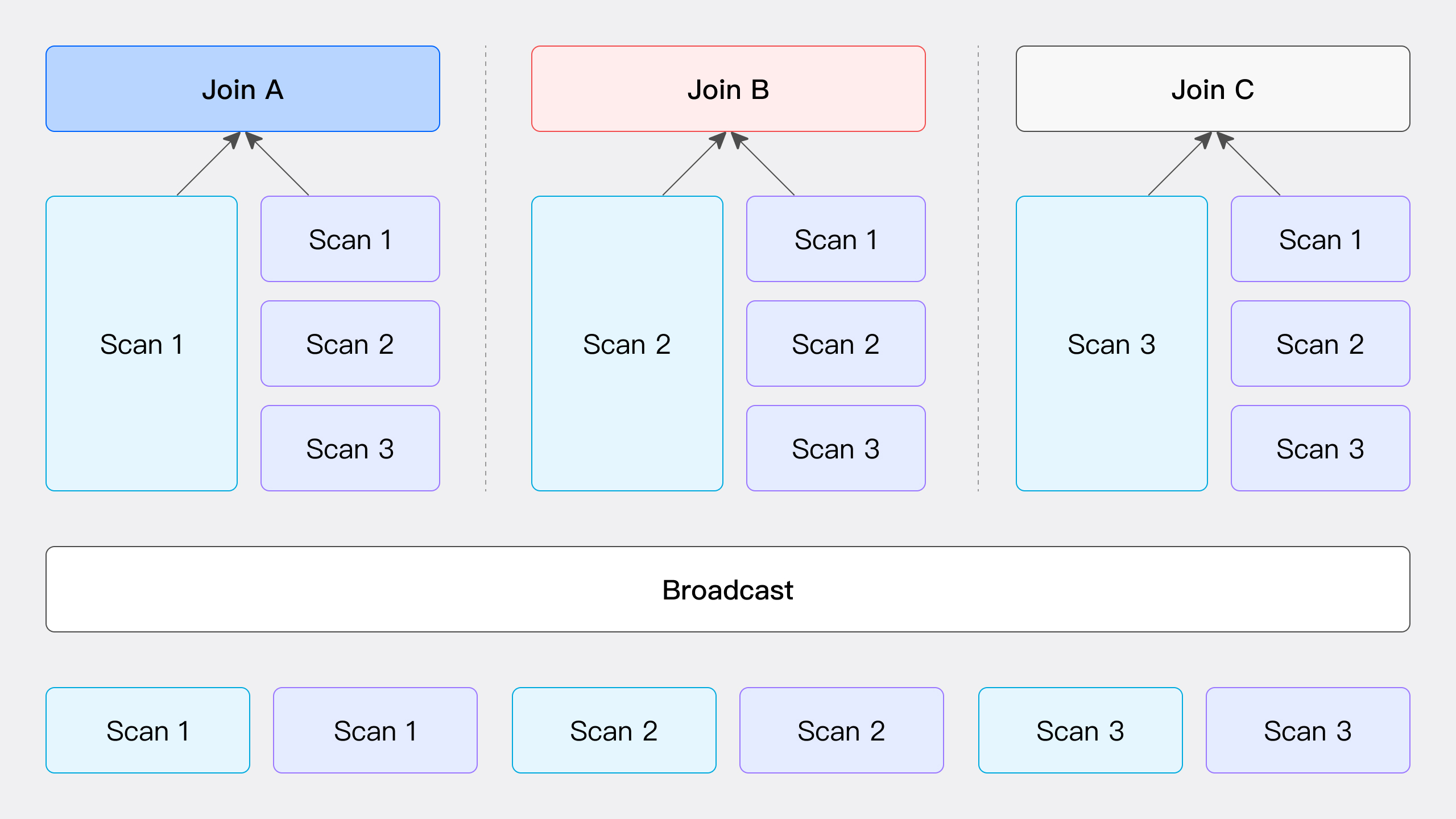
As shown in the figure, Broadcast Join involves sending all the data from the right table to all nodes participating in the JOIN computation, including the nodes scanning the left table data, while the left table data remains stationary. Each node receives a complete copy of the right table's data (total data volume T(R)), ensuring that all nodes have the necessary data to perform the JOIN operation.

This method is suitable for a variety of general scenarios but is not applicable to RIGHT OUTER, RIGHT ANTI, and RIGHT SEMI types of Hash Join. The network overhead is the number of JOIN nodes N multiplied by the right table's data volume T(R).

Partition Shuffle: The Conventional Approach

Partition Shuffle employs a bidirectional distribution strategy, hashing and distributing both tables based on the JOIN key. The network overhead equals the sum of the data volumes of the two tables. This method is like Tai Chi, emphasizing balance, and is suitable for scenarios where the data volumes of the two tables are similar.

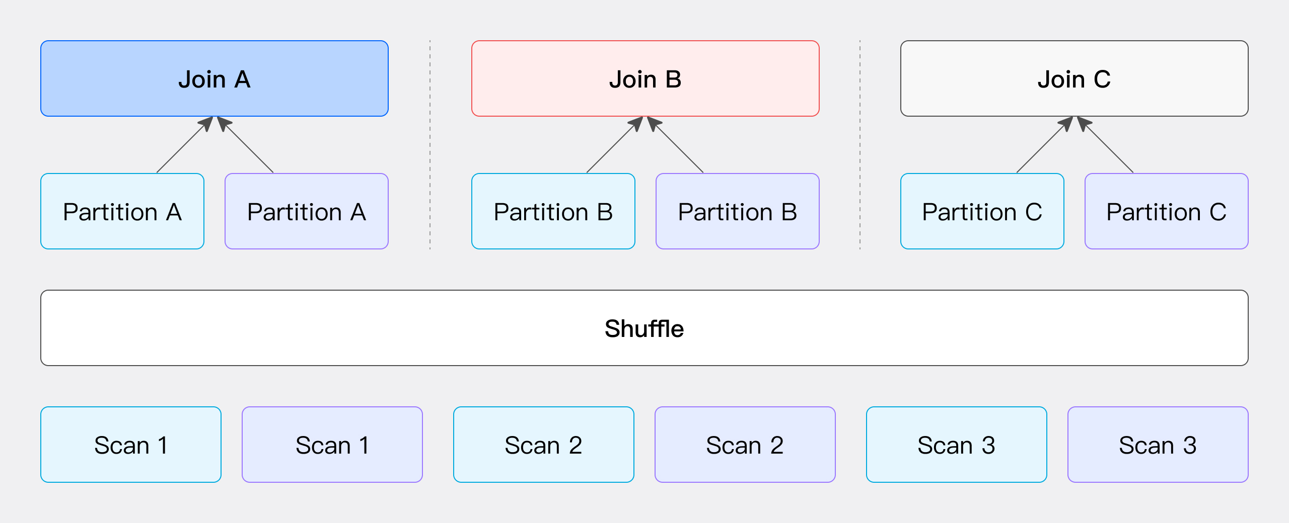
This method involves calculating hash values based on the JOIN condition and partitioning the data accordingly. Specifically, the data from both the left and right tables is partitioned based on the hash values calculated from the JOIN condition and then sent to the corresponding partition nodes (as shown in the figure).

The network overhead for this method includes the cost of transmitting the left table's data T(S) and the cost of transmitting the right table's data T(R). This method only supports Hash Join operations because it relies on the JOIN condition to perform data partitioning.

Bucket Shuffle: The Cost-Effective Approach

Bucket Shuffle leverages the bucketing characteristics of the tables, requiring redistribution of only the right table's data. The network overhead is merely the data volume of the right table. It's like a martial artist using the opponent's strength against them, making good use of their advantages. This method is particularly efficient when the left table is already bucketed by the JOIN key.

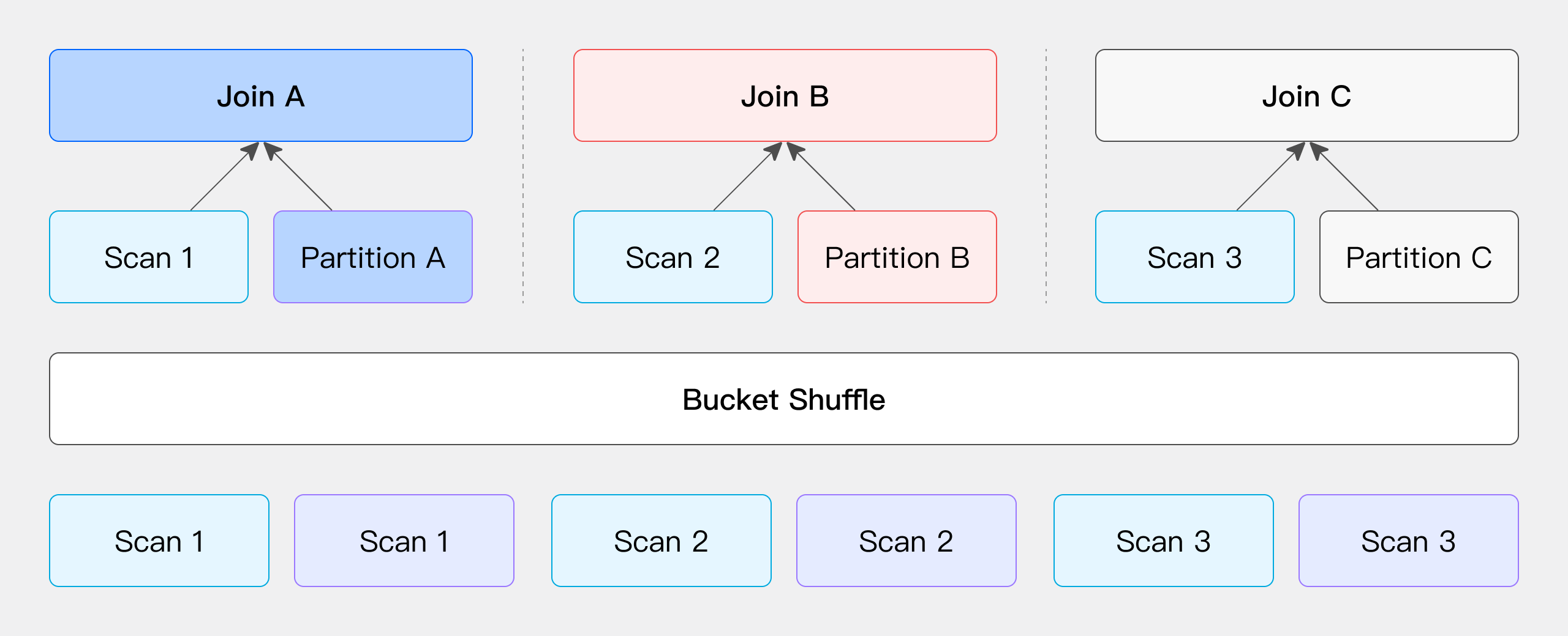
When the JOIN condition includes the bucketing column of the left table, the left table's data remains stationary, and the right table's data is redistributed to the left table's nodes for JOIN, reducing network overhead.

When one side of the table participating in the JOIN operation has data that is already hash-distributed according to the JOIN condition column, we can choose to keep the data location of this side unchanged and only move and redistribute the other side of the table. (Here, the "table" is not limited to physically stored tables but can also be the output result of any operator in an SQL query, and we can flexibly choose to keep the data location of the left or right table unchanged and only move the other side.)

Taking Doris' physical tables as an example, since the table data is stored through hash distribution calculations, we can directly use this characteristic to optimize the data shuffle process during JOIN operations. Suppose we have two tables that need to be JOINed, and the JOIN column is the bucketing column of the left table. In this case, we do not need to move the left table's data; we only need to redistribute the right table's data according to the left table's bucketing information to complete the JOIN calculation (as shown in the figure).

The network overhead for this process mainly comes from the movement of the right table's data, i.e., T(R).

Colocate Join: The Ultimate Expert

Colocate Join is the ultimate optimization, where data is pre-distributed in the same manner, and no data movement is required during JOIN. It's like a perfectly synchronized partnership, with seamless cooperation. Zero network overhead and optimal performance, but it has the strictest requirements.

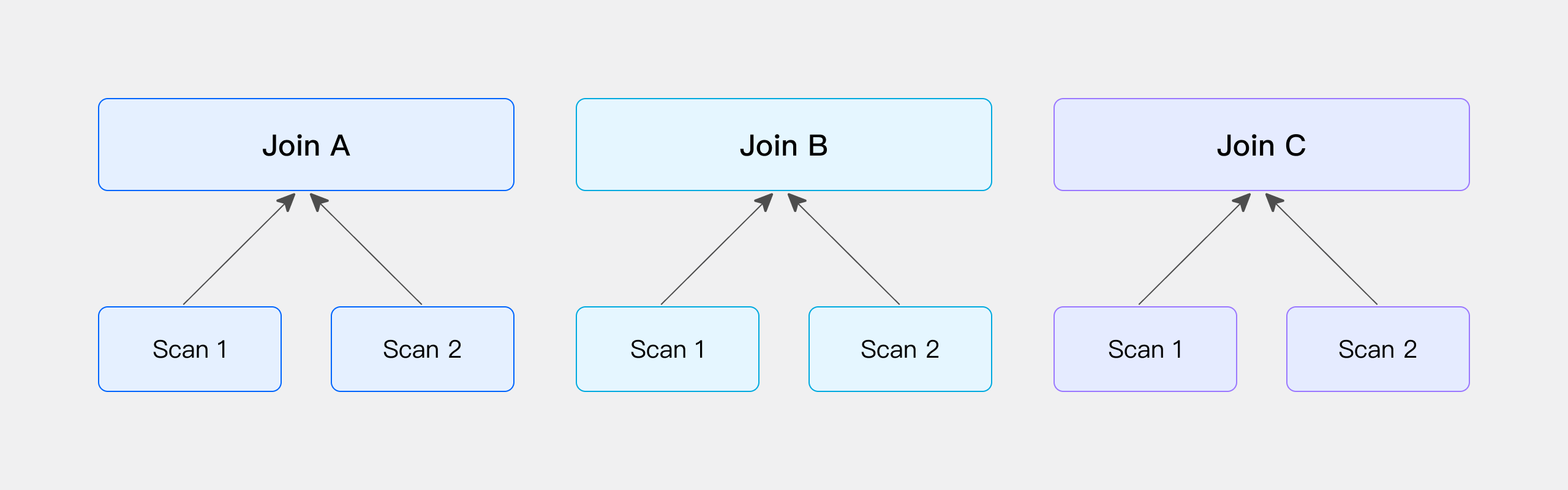
Similar to Bucket Shuffle Join, if both sides of the table participating in the JOIN are hash-distributed according to the JOIN condition column, we can skip the shuffle process and directly perform the JOIN calculation locally. Here is a simple illustration using physical tables:

When Doris creates tables with DISTRIBUTED BY HASH, the data is distributed according to the hash distribution key during data import. If the hash distribution key of the two tables happens to match the JOIN condition column, we can consider that the data of these two tables has been pre-distributed according to the JOIN requirements, i.e., no additional shuffle operation is needed. Therefore, during actual querying, we can directly perform the JOIN calculation on these two tables.

Colocate Join Example

After introducing the four types of Hash Join in Doris, let's pick Colocate Join, the ultimate expert, for a showdown:

In the example below, both tables t1 and t2 have been processed by the GROUP BY operator and output new tables (at this point, both tx and ty are hash-distributed according to c2). The subsequent JOIN condition is tx.c2 = ty.c2, which perfectly meets the conditions for Colocate Join.

explain select *
from 
    (
        -- Table t1 is hash-distributed by c1. After the GROUP BY operator, the data distribution becomes hash-distributed by c2.
        select c2 as c2, sum(c1) as c1
        from t1
        group by c2 
    ) tx
join 
    (
        -- Table t2 is hash-distributed by c1. After the GROUP BY operator, the data distribution becomes hash-distributed by c2.
        select c2 as c2, sum(c1) as c1
        from t2
        group by c2 
    ) ty
on tx.c2 = ty.c2;

From the Explain execution plan result below, we can see that the left child node of the 8th Hash Join node is the 7th aggregation node, and the right child node is the 3rd aggregation node, with no Exchange node appearing. 

This indicates that the data from both the left and right child nodes after aggregation remains in its original location without any data movement and can directly perform the subsequent Hash Join operation locally.

+------------------------------------------------------------+

| Explain String(Nereids Planner)                            |

+------------------------------------------------------------+

| PLAN FRAGMENT 0                                            |

|   OUTPUT EXPRS:                                            |

|     c2[#20]                                                |

|     c1[#21]                                                |

|     c2[#22]                                                |

|     c1[#23]                                                |

|   PARTITION: HASH_PARTITIONED: c2[#10]                     |

|                                                            |

|   HAS_COLO_PLAN_NODE: true                                 |

|                                                            |

|   VRESULT SINK                                             |

|      MYSQL_PROTOCAL                                        |

|                                                            |

|   8:VHASH JOIN(373)                                        |

|   |  join op: INNER JOIN(PARTITIONED)[]                    |

|   |  equal join conjunct: (c2[#14] = c2[#6])               |

|   |  cardinality=10                                        |

|   |  vec output tuple id: 9                                |

|   |  output tuple id: 9                                    |

|   |  vIntermediate tuple ids: 8                            |

|   |  hash output slot ids: 6 7 14 15                       |

|   |  final projections: c2[#16], c1[#17], c2[#18], c1[#19] |

|   |  final project output tuple id: 9                      |

|   |  distribute expr lists: c2[#14]                        |

|   |  distribute expr lists: c2[#6]                         |

|   |                                                        |

|   |----3:VAGGREGATE (merge finalize)(367)                  |

|   |    |  output: sum(partial_sum(c1)[#3])[#5]             |

|   |    |  group by: c2[#2]                                 |

|   |    |  sortByGroupKey:false                             |

|   |    |  cardinality=5                                    |

|   |    |  final projections: c2[#4], c1[#5]                |

|   |    |  final project output tuple id: 3                 |

|   |    |  distribute expr lists: c2[#2]                    |

|   |    |                                                   |

|   |    2:VEXCHANGE                                         |

|   |       offset: 0                                        |

|   |       distribute expr lists:                           |

|   |                                                        |

|   7:VAGGREGATE (merge finalize)(354)                       |

|   |  output: sum(partial_sum(c1)[#11])[#13]                |

|   |  group by: c2[#10]                                     |

|   |  sortByGroupKey:false                                  |

|   |  cardinality=10                                        |

|   |  final projections: c2[#12], c1[#13]                   |

|   |  final project output tuple id: 7                      |

|   |  distribute expr lists: c2[#10]                        |

|   |                                                        |

|   6:VEXCHANGE                                              |

|      offset: 0                                             |

|      distribute expr lists:                                |

|                                                            |

| PLAN FRAGMENT 1                                            |

|                                                            |

|   PARTITION: HASH_PARTITIONED: c1[#8]                      |

|                                                            |

|   HAS_COLO_PLAN_NODE: false                                |

|                                                            |

|   STREAM DATA SINK                                         |

|     EXCHANGE ID: 06                                        |

|     HASH_PARTITIONED: c2[#10]                              |

|                                                            |

|   5:VAGGREGATE (update serialize)(348)                     |

|   |  STREAMING                                             |

|   |  output: partial_sum(c1[#8])[#11]                      |

|   |  group by: c2[#9]                                      |

|   |  sortByGroupKey:false                                  |

|   |  cardinality=10                                        |

|   |  distribute expr lists: c1[#8]                         |

|   |                                                        |

|   4:VOlapScanNode(345)                                     |

|      TABLE: tt.t1(t1), PREAGGREGATION: ON                  |

|      partitions=1/1 (t1)                                   |

|      tablets=1/1, tabletList=491188                        |

|      cardinality=21, avgRowSize=0.0, numNodes=1            |

|      pushAggOp=NONE                                        |

|                                                            |

| PLAN FRAGMENT 2                                            |

|                                                            |

|   PARTITION: HASH_PARTITIONED: c1[#0]                      |

|                                                            |

|   HAS_COLO_PLAN_NODE: false                                |

|                                                            |

|   STREAM DATA SINK                                         |

|     EXCHANGE ID: 02                                        |

|     HASH_PARTITIONED: c2[#2]                               |

|                                                            |

|   1:VAGGREGATE (update serialize)(361)                     |

|   |  STREAMING                                             |

|   |  output: partial_sum(c1[#0])[#3]                       |

|   |  group by: c2[#1]                                      |

|   |  sortByGroupKey:false                                  |

|   |  cardinality=5                                         |

|   |  distribute expr lists: c1[#0]                         |

|   |                                                        |

|   0:VOlapScanNode(358)                                     |

|      TABLE: tt.t2(t2), PREAGGREGATION: ON                  |

|      partitions=1/1 (t2)                                   |

|      tablets=1/1, tabletList=491198                        |

|      cardinality=10, avgRowSize=0.0, numNodes=1            |

|      pushAggOp=NONE                                        |

|                                                            |

|                                                            |

| Statistics                                                 |

|  planed with unknown column statistics                     |

+------------------------------------------------------------+

105 rows in set (0.06 sec)

The Path to JOIN Decision

After listening to Old Li's explanation, Xiao Zhang had an epiphany. JOIN optimization is not about simply choosing one solution; it's about making flexible decisions based on the actual situation:

Joining a large table with a small table?
Go all-in with Broadcast Join.

Tables of similar size?
Partition Shuffle is a safe bet.

Left table bucketed appropriately?
Bucket Shuffle shows its power.

Joining tables in the same group?
Colocate Join leads the way.

Non-equi-JOIN?
Nest Loop Join comes to the rescue.

After putting these strategies into practice, Xiao Zhang compiled a set of JOIN optimization tips:

• Plan data distribution in advance to lay the foundation for high-performance JOIN operations.
• Leverage partition pruning to reduce the amount of data involved in JOINs.
• Design bucketing strategies wisely to create favorable conditions for Bucket Shuffle and Colocate Join.
• Configure parallelism and memory properly to maximize JOIN performance.
• Monitor resource usage closely to identify performance bottlenecks in a timely manner.

By optimizing queries based on these insights, Xiao Zhang was able to reduce tasks that originally took hours to just a few minutes, earning high praise from his boss.

The world of JOIN optimization is vast and complex; what we've explored today is just the tip of the iceberg. Choosing the right JOIN strategy for different scenarios is key to finding the optimal balance between performance and resource consumption.